Automated Spectral QA · HSI · MSI · Thermal · EO · Point

Bad spectral data
is invisible.
Until now.

Sensor data integrity and quality checks for spectral instruments: hyperspectral, multispectral, thermal, EO and point. Today they happen retroactively, if at all, and cost hours you have already spent. SpectrIQ runs them at capture, against the physics of the instrument that made the data, and writes what it found into a report you keep.

Download the free 60-day trial See how it works →
$2K–6K To re-task one failed satellite collection
46 Checks in the imaging suite; thermal, EO and point route to their own
890 Tests passing in the engine

Watch SpectrIQ catch what other tools miss.

A four-minute walkthrough of the QA pipeline running on real MicaSense RedEdge captures, flagging illumination drift, incomplete bands and silent spectral corruption as the capture comes in.

Detect. Explain. Decline.

Saturation, calibration drift and illumination instability look identical to good data on any standard preview, until an analyst opens the cube days later. SpectrIQ closes that gap at acquisition time, and tells the operator what it found.

01
Closed-Loop QA

46 checks on an imaging capture, each rated

Exposure, signal-to-noise, calibration drift, spectral shape, geometry, detector health, each rated Advisory, Degraded, Severe or Fatal, each carrying a stated remedy. The output is advisory. Nothing is suppressed, deleted or withheld, and an operator decides what to do about it.

02
Honest Accounting

A check that cannot run says so

On a delivered orthomosaic most of the suite declines: no dark reference, no integration time, no scan line. In a full run every module in the baseline suite is accounted for: it executes, or it is recorded not-applicable with a stated reason. Some runs shown below used a reduced selection of checks, and each card says how many ran. A clean bill of health and a short one are different things, and the report tells them apart.

03
Edge & Ground Station

Runs offline, where the data is

A Python pipeline with YAML-driven configuration that runs on a laptop or ground station with no cloud and no network. Adding a camera in a format the engine already reads is a config file; a new product format needs a loader. Five sensor classes route to four check registries. Hyperspectral and multispectral share the imaging suite (46 checks), thermal/IR has its own (41), EO/RGB its own (16), and a non-imaging point spectrometer its own (4), so a capture is routed to the checks written for its sensor class.

Five published public datasets.
Two had a defect in the delivered product.

USGS, USACE/JALBTCX, NOAA, USGS/NASA and NSF NEON: 10-band multispectral, 48-band and 426-band hyperspectral, 3-band RGB and single-band thermal. Two of the five turned up a defect in the delivered metadata; the other three came back without a confirmed defect, and we say so rather than reach for a finding. Every dataset here is publicly released and credited below.

USGS EROS Cal/Val · ECCOE 2023

PASS 88.1

MicaSense RedEdge-MX Dual · 10-band multispectral

Sampled at the field spectrometer’s recorded GPS positions, the orthomosaic differs in spectral shape from the field spectra at the five brightest points by 33.6°, against a 12° limit, so SpectrIQ set that comparison aside rather than report it. That is consistent with the roughly 12 m horizontal accuracy the release documents for those GPS fixes, against 4 cm pixels; it is not a defect in the release. Extra calibration work did not beat the manufacturer default on this dataset. A reduced run: 3 of the 46 imaging checks were selected for this capture.
USACE / JALBTCX · NCMP 2019 & 2018

5 PASS

Itres CASI-1500 · 48-band hyperspectral

Each sidecar carries three extent records. Two locate the raster correctly; the third is an unpopulated template default: the same fixed box near Stanwood, Washington in every sidecar inspected, across two deliveries in different years and different states. Because the box is fixed and the imagery is not, how far wrong it reads depends on the delivery: about 3,040 km for the Alaska tiles, about 3,520 km for the New York ones. It is the GeoBndBox at dataIdInfo/dataExt/geoEle with no esriExtentType attribute (the standard ISO 19115 path, which is the one a consumer reads), and is checkable in about ninety seconds. A packaging defect in the discovery metadata, not an imagery one: the GeoTIFF georeferencing is correct and the imagery is fully usable. And the same square kilometre, published twice, disagrees by a median 16.5% per band, in relative digital number; no radiometric units are declared. That is SpectrIQ’s figure, from a blind run; a separate manual analysis of the same pair landed at 16.2%. A reduced run: 11 of the 46 imaging checks were selected for these tiles.

USACE NCMP Phase One + NOAA NGS · 2022 & 2017–20

3 PASS

RGB framing camera + DSS natural colour · 3-band

No defects found in the imagery. Worth passing on: the two Portland years ship in different coordinate reference systems: same zone, same pixel, different datum declaration.

USGS / NASA · Landsat 8–9 TIRS 2024

5 PASS

Surface temperature · single-band thermal

No defects found in the data: five windows over Phoenix and Lake Mead, all passing, including one placed deliberately across the swath edge to see whether any check would read fill as measured ground. On a calibrated satellite product 13 of the thermal suite’s 41 checks can execute; the rest decline, each with its reason, because the sensor state they need is not in a delivered product.

NSF NEON · AOP 2017 & 2018

6 PASS

NEON Imaging Spectrometer · 426-band hyperspectral

The widest product yet: 426 bands, 380–2510 nm, and three different spectrometers across two collection years. All six captures pass. One check, Spectral Smoothness, flags every capture as advisory: 15–21% of pixels carry spectral spikes, concentrated in the bluest bands near 380–410 nm, and the cause is not yet classified. The same ground in two collection years differs by a median 6.9–11.4% per band in reflectance; the years were flown by different instruments, so that difference is measured but not attributed. NEON publishes more of what the checks need than any product here: band centres, per-band FWHM, a declared scale factor, a declared fill value and a per-pixel atmospheric classification, all inside the delivered file. A small number of metadata observations go to NEON before they are published anywhere.

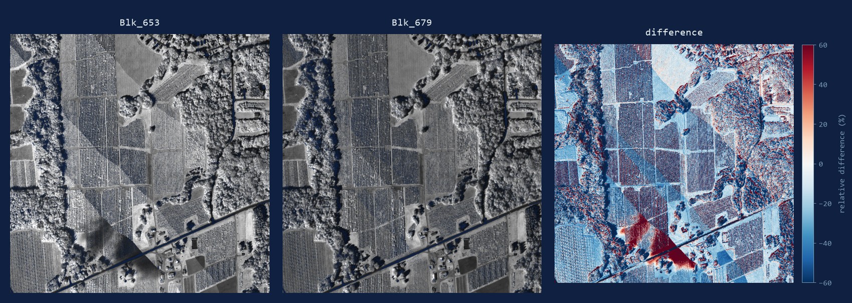
Three panels. The left two are near-identical greyscale near-infrared renderings of the same one-square-kilometre tile, published under two different collection blocks. The right panel maps the difference between them and is strongly patterned, with straight diagonal boundaries that do not follow any ground feature.
The same square kilometre, published twice. Some Lake Ontario tiles ship under two collection blocks, flown one day apart. The two renderings look identical; their difference does not. It is organised into straight-edged regions that cut across fields, treelines and the road, so it is not ground change. Across 989,081 stable co-located pixels, SpectrIQ puts the median per-band difference at 16.5%, in relative digital number; the delivery declares no radiometric units. A separate manual analysis of the same pair found 16.2%.
+24.5% mean · bands 0–15 −20.1% mean · bands 32–47 +80+60+40+20+0−20081624324047 band index · wavelength increases left to right relative difference (%)
And it depends on wavelength. SpectrIQ puts the first third of the bands 24.5% higher in one publication and the last third 20.1% lower, a 44.6 pp spread, by band index because the delivery publishes no band centres. An exposure offset would move every band the same way; this does not. The change is not steady across the spectrum: it flattens and partly reverses in the middle bands. Two rasters cannot say whether the cause is view geometry or atmospheric correction, so SpectrIQ reports it as measured and leaves it undetermined.

Data sources. ECCOE imagery: U.S. Geological Survey, EROS Cal/Val Center of Excellence and National Uncrewed Systems Office, public release, doi:10.5066/P14FFHW5. NCMP imagery: U.S. Army Corps of Engineers Joint Airborne Lidar Bathymetry Technical Center of eXpertise (JALBTCX), National Coastal Mapping Program, via NOAA Digital Coast (access constraints: none). EO imagery: USACE NCMP Phase One and NOAA National Geodetic Survey, via NOAA Digital Coast. Thermal imagery: Landsat 8–9 Collection 2 Level-2 data courtesy of the U.S. Geological Survey. NEON imagery: this material is based in part upon work supported by the National Ecological Observatory Network (NEON), a program sponsored by the U.S. National Science Foundation (NSF) and operated under cooperative agreement by Battelle.

A failed capture costs differently
in every vertical. None of them cheaply.

Spectral science and spectral imagery analysis is the market SpectrIQ serves, and it sits inside a $103B geospatial analytics market growing to $234B by 2033, with earth-observation services alone at $7B and roughly doubling by 2034.1 What a bad capture costs depends entirely on who is flying, and in every case nobody finds out at acquisition time, when it is still cheap to fix.

HSI + MSI

Defense & UAV

ISR in contested environments. The collection is rarely the expensive part; the analyst hours spent on it are, at roughly $37/hour loaded for a GEOINT imagery analyst, and a bad capture burns them before anyone knows.2 A failed acquisition is not a re-fly you schedule: it is a re-tasking, an exposure, and sometimes a window that does not come back.

MSI dominant

Precision Agriculture

Commercial survey flights run $1,500–$10,000 per mission, with project minimums near $3,000 and photogrammetry billed at $150–$300 per acre.3 A miscalibrated flight is that cost again, plus mobilisation. At worst the crop has moved on and the treatment window closed while the data looked fine.

HSI + MSI

Pharma & Food QC

A bad capture here is a batch decision and an audit finding, not a re-shoot. Structured QA output maps directly to 21 CFR Part 11 audit trails: compliance enabler, not cost.

MSI dominant

Satellite & EO

New tasking runs $40–$60/km² for sub-metre imagery against a 50–100 km² minimum order, so a failed collection is roughly $2,000–$6,000 to buy again, days or weeks later.4 Multi-temporal calibration consistency is the unsolved quality problem here.

Figures, so they can be checked. All figures below are third-party. Costs vary by provider, region and contract; treat them as orders of magnitude rather than quotes.
  1. Geospatial analytics market USD 102.7B (2025), Grand View Research; earth observation USD 7.04B (2025) to USD 14.55B (2034), Fortune Business Insights. The hyperspectral imaging systems market specifically is far smaller: about USD 0.9–1.8B in 2025 depending on scope.
  2. Geospatial intelligence imagery analyst, USD 37.32/hour average, Salary.com. Fully loaded contractor rates run higher.
  3. Drone survey pricing, Northern Drone and UAV Sphere.
  4. Very-high-resolution new tasking USD 40–60/km² with 50–100 km² minimum orders; archive imagery 40–60% less, OnGeo Intelligence and Geopera. Providers differ; treat as an order of magnitude, not a quote.

The quality gap is real.
The layer that closes it is unoccupied.

SpectrIQ is patent pending and in active development. If you operate hyperspectral or multispectral sensors and want early access, or if you're an investor interested in the spectral imaging infrastructure space, we'd like to hear from you.

info@spectriq.io